I recently implemented V1 of Racing SLAM, a monocular visual SLAM algorithm intended for car racing footage. It took about a full one to two weeks of work, but I’m relieved to have something that works… kinda. There’s still issues with V1; it doesn’t seem to work well on footage with complex motion. But I still believe there’s value in getting it to work on simple footage with forwards motion. It means that something is working. When solving a hard problem, that usually a good first step. Get something working. V2 will be a whole other story. There’s a lot of rethinking that needs to happen. For now, here’s a brief overview of how V1 works.
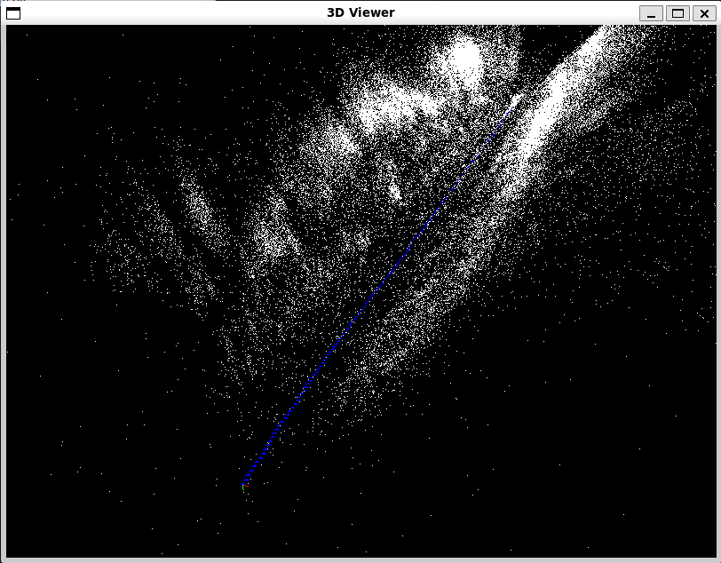
 A map built from footage of a car driving down a highway lined with trees.
Overview
WARNING
This section is technical
1. Features
V1 uses visual features identified in the image using a modified version of the Harris corner detector. For each feature, an ORB (BRIEF) descriptor is computed. These features are matched with the features in the previous frame using nearest neighbor and Lowe’s ratio test to filter matches.
2. Pose Estimation
Consecutive frame feature matches are then used to compute the essential matrix, and outlier points are discarded using RANSAC. Four different pose hypotheses can be recovered from the essential matrix and the most probable configuration is chosen: probability is determined based on the number of triangulated features that lie in front of both cameras. The pose is then used as the initial estimate for the frame.
3. Pose Optimization
The 3D map point correspondences from the previous frame are copied over to the corresponding features in the new frame. Then, a pose graph optimization occurs to minimize the reprojection error by optimizing only the current pose. This takes the form of a non-linear least squares problem which is solved using the Levenberg-Marquardt algorithm.
4. Map Matching
Further correspondences between image features and existing map points are searched by projecting the map points onto the image plane. The projected points are matched to features with a close pixel distance and a low ORB distance.
5. Triangulation
Any features that were matched with the previous frame, but not matched with map points are then triangulated and added to the 3D map.
6. Local Bundle Adjustment
Every 5 frames, bundle adjustment is performed. This is an algorithm similar to pose graph optimization, but both 3D map point locations and poses are optimized concurrently. The last 10 poses are optimized, along with all map points observed from any of those ten frames. This helps correct triangulated points and pose drift.
7. Culling
Finally, map points with poor reprojection error are removed from the map. Points that haven’t been observed recently and that have few observations in total are also removed. This keeps the map smaller and reduces noise.